Introduction
Our project is to explore both Markov Chain Monte Carlo algorithms and variational inference methods for Latent Dirichlet Allocation (LDA). This blog is meant to be used by a consumer-facing or general audience, and so we will skip the technical details and give a high-level plain language explanation. For more technical details, please refer to our final paper.
Latent Dirichlet Allocation (LDA)
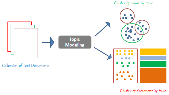
Latent Dirichlet Allocation (LDA) is a model that describes how collections of discrete data are generated and tagged. For our purposes, we will focus on text documents about various topics. For example, every Wikipedia page can be considered as a document and each document would be about several topics, such as politics, soccer, history, music, and so on.
We are interested in learning about these topics in an unsupervised manner -- in other words, without humans giving hints or suggestions as to what the topics are. To do get there, we need (1) an underlying model of how documents with their topics are generated, and (2) given this model, fit the parameters with actual live data. LDA would be the solution to the first problem.
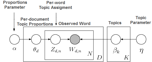
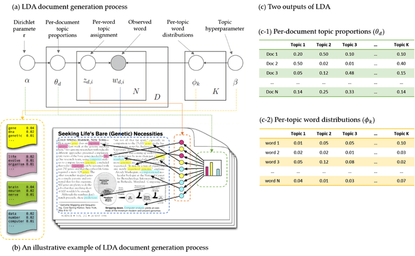
Firstly, don’t be alarmed by the many symbols. We can get through this together. What we actually observe is the words on every Wikipedia article. This is represented by the gray circle, with the subscripts denoting which Wikipedia article and word in that article we observe. Everything else in this model is latent variables, that is, not directly observed. Our goal is to infer what these variables are through their collective impact on the observed words.
The rectangles around the circles represent multiplicity. There are N words in every document, and there are D documents in total. There are also K topics.
You might also notice that there are two pathways to determine the word in every document. The pathway on the left determines the topic assignment. Is this word about “music” or “sports”, for example? The right pathway determines the word in the vocabulary of the topic. If the topic assignment is “sports”, the vocabulary might consist of words such as “goals”, “soccer”, and “score”, for example.
Topic Assignment
Starting from the far left, alpha is a hyperparameter that determines how concentrated the topics are. Would a random Wikipedia document discuss many topics, or would it focus on a small number of topics? Typically, it does not make sense that a document would talk about everything under the sun, and so we will expect some concentration of topics as a good author is wise to focus his or her energies.Next, based on alpha and the Dirichlet distribution, each document receives its own theta value which determines the overall proportion of topics in the document. (We can see now that we have D thetas as we enter the rectangle marked D) Perhaps one theta value might be 50% “health” and 50% “food”, if the article is about the healing ability of good cooking!
Next, based on theta and the multinomial distribution, each word in every document receives its own topic assignment, making D x N assignments in total. The model is a bag of words, so the ordering does not matter. Based on our previous example of 50% “health” and 50% “food”, each word would be flipping a coin and getting exactly only one of those assignments.
Topic Vocab
From the above, we have topic assignments for every word in every document. How is the actual word chosen? Starting from the far right, we have another hyperparameter of the Dirichlet distribution, to determine the concentration of the vocabulary of each topic. Since there are K topics, we draw from the Dirichlet distribution K times to get a discrete probability distribution of the vocabulary of each topic. For example, if the topic is “food”, the probabilities of words such as “sushi”, “rice”, “egg” would be higher than other topics.Putting it together, we will condition on the chosen topic for the word from the topic assignment on the left pathway. This looks up the appropriate vocabulary for that topic. Using another multinomial distribution, we basically roll a weighted die customized for that topic to choose a random word assignment. This results in actual words that we observe.
This process is called Latent Dirichlet Allocation. The term “latent” refers to the fact that many of the parameters cannot be observed directly. The term “Dirichlet Allocation” refers to the manner in which we assign discrete probabilities on topic proportions.
Visualizing the document generative process
Bayesian Inference
Now that we have a generative model on how documents are generated from topics, the next step is to fit the model on live data. This process is called Bayesian Inference, which maximizes the likelihood of the latent parameters to match what we have seen from live data.The issue is that solving this problem is intractable. This means it is difficult or impossible to solve analytically. The problem arises from the dependence of variables from the two pathways of “Topic Assignment” and “Topic Vocab”, where solving each pathway would require knowledge of the other.
Instead of trying to find the exact solution, it would thus be better to find a good approximate solution. Along this line, Mean-field variational inference and Gibbs Sampling are two popular ways to solve the inference problem for the latent parameters.
Mean-field variational inference
Variational inference
The technical term for the correct distribution given the observed data is the posterior, denoted by P, which is often not a “nice” distribution to deal with mathematically. The posterior can be any distribution at all and doesn’t have to be a well-known distribution that is mathematically easy to manipulate. The solution is to choose a distribution Q from a user-defined variational family that approximates P. (We choose Q within the variational family that is “closest” to P, using measures such as KL divergences.) This process of choosing a variational family, and then finding the closest distribution Q to P within that variational family is known as variational inference.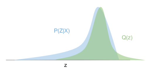
Mean-field variational inference
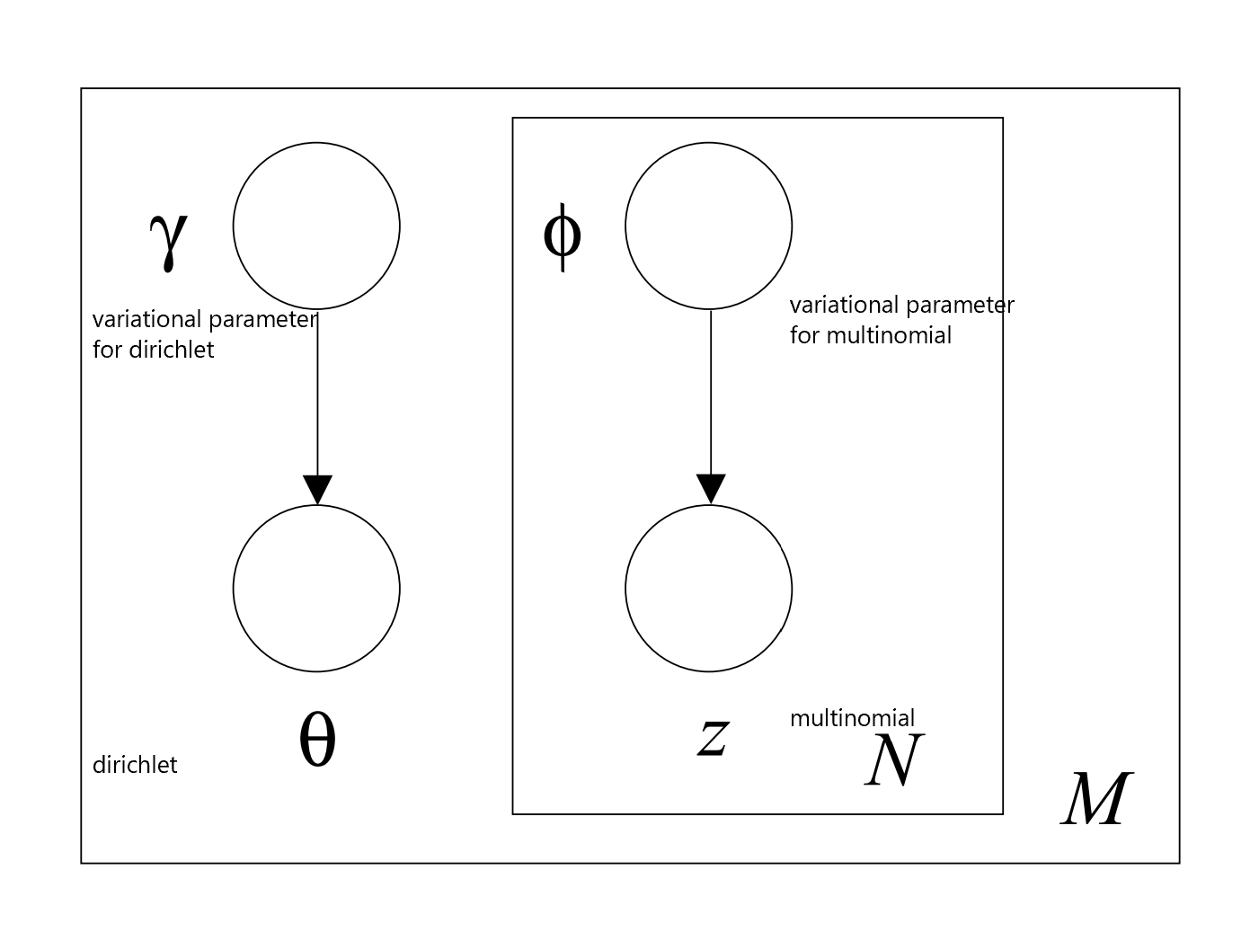
Mean-field variational inference is a special case of variational inference where we further assume that the variational family can be fully factored. In other words, the latent parameters are all independent of each other. Recall that our main problem was due to the dependence of the variables on the left and right pathways to the observed data, with conditional probabilities involved in the definition. If we instead choose to break this and assume independence, the variational family would not have to deal with conditional probabilities but instead, be simply the product of all the multinomial and Dirichlet distributions. Explicitly: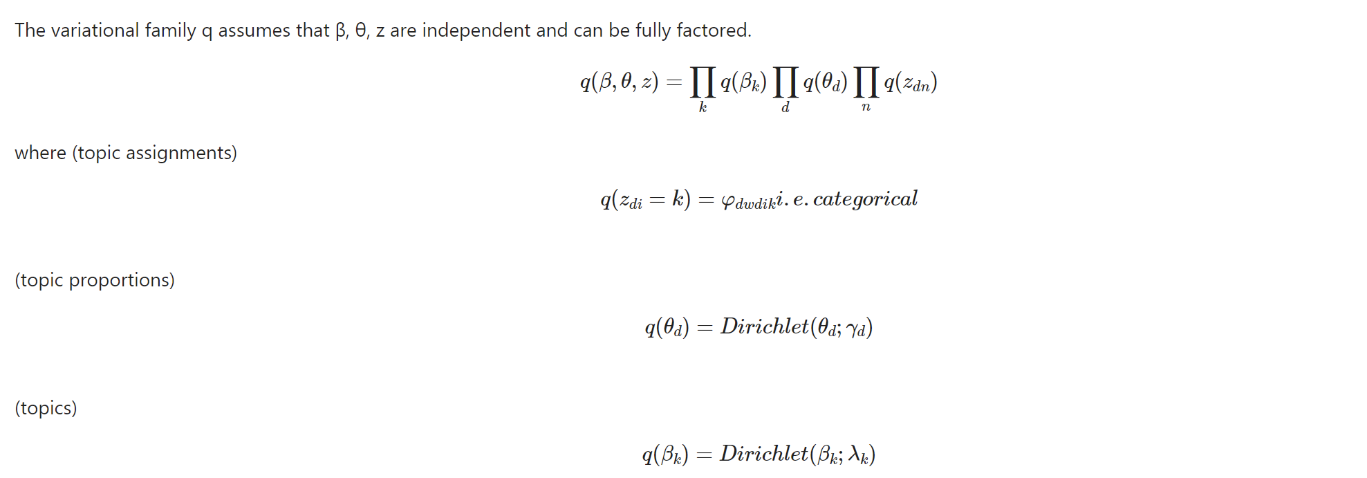
Then, the M step matches the beta from the right pathway for topic vocab, while again assuming that the latent parameters from the E step are correct due to independence. (This is done by optimizing the variational parameters of lambda for beta.)
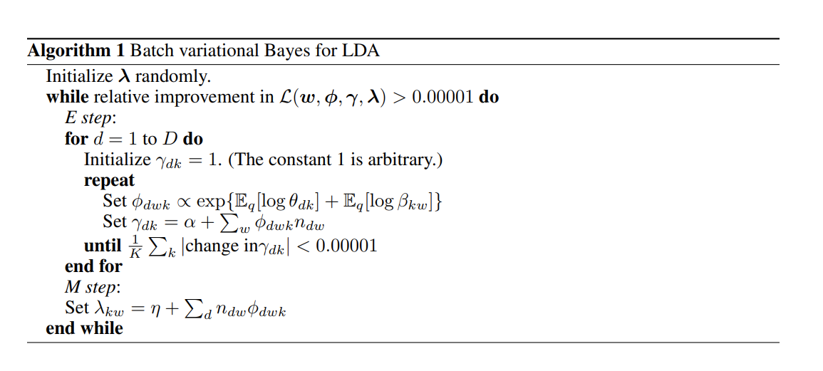
The pseudo-code of the EM algorithm is shown below.
Gibbs Sampling
In Q1 we explored MCMC methods, specifically the Metropolis-Hastings algorithm, to solve the problem of computing high-dimensional integrals. We learned that this particular class of sampling methods was especially effective in performing probabilistic inferences which can be applied to solve problems specifically within the field of Bayesian inference and learning. We applied this particular MCMC method for sampling posterior distributions, since the posterior probability distribution for parameters given our observations proved to be intractable, hence the use of sampling algorithms for approximate inference.
LDA is similar in that its aim is to infer the hidden structure of documents through posterior inference. Since we cannot exactly compute the conditional distribution of the hidden variables given our observations, we can use MCMC methods to approximate this intractable posterior distribution. Specifically, we can use Gibbs sampling to implement LDA. Gibbs sampling is another MCMC method that approximates intractable probability distributions by consecutively sampling from the joint conditional distribution: \[ P(W,Z,\phi, \theta| \alpha, \beta).\] This models the joint distribution of topic mixtures $\theta$, topic assignments $Z$, the words of a corpus $W$, and the topics $\phi$. In the approach we use, we leverage the collapsed Gibbs sampling method in not representing $\phi$ or $\theta$ as parameters to be estimated, and only considering the posterior distribution over the word topic assignments $P(Z|W)$.
The first step of the algorithm is to go through each document and randomly assign each word in the document to one of the K topics. Apart from generating this topic assignment list, we’ll also create a word-topic matrix, which is the count of each word being assigned to each topic. And a document-topic matrix, which is the number of words assigned to each topic for each document (distribution of the topic assignment list)
The initialization of random assignments gives you both the topic representations of all the documents and word distributions of all the topics, though not very good ones. In order to improve and eventually compute more accurate estimates of our parameters, we’ll employ the collapsed gibbs sampling method that performs the following steps for fixed number of iterations:
- Reassign a new topic to w, where we choose a new topic assignment from the full conditional distribution:
Sampling from this distribution allows us to retrieve more accurate topic assignments as the sampler runs. Note $C^{WT}$ is the word-topic matrix, and $C^{DT}$ is the document-topic matrix.
After updating the topic assignments for the word tokens we can also retrieve estimates for the theta and phi parameters using the topic allocations.
By estimating the parameters phi and theta we have effectively accomplished our goals in estimating which words are important for which topic and which topics are important for a particular document, respectively.
Our approaches
Data Preprocessing
Experiments
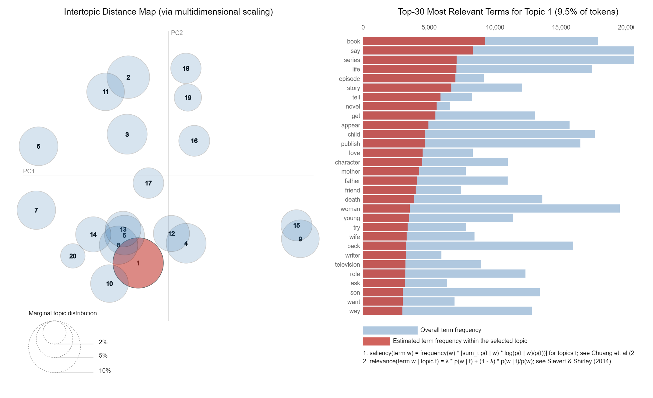
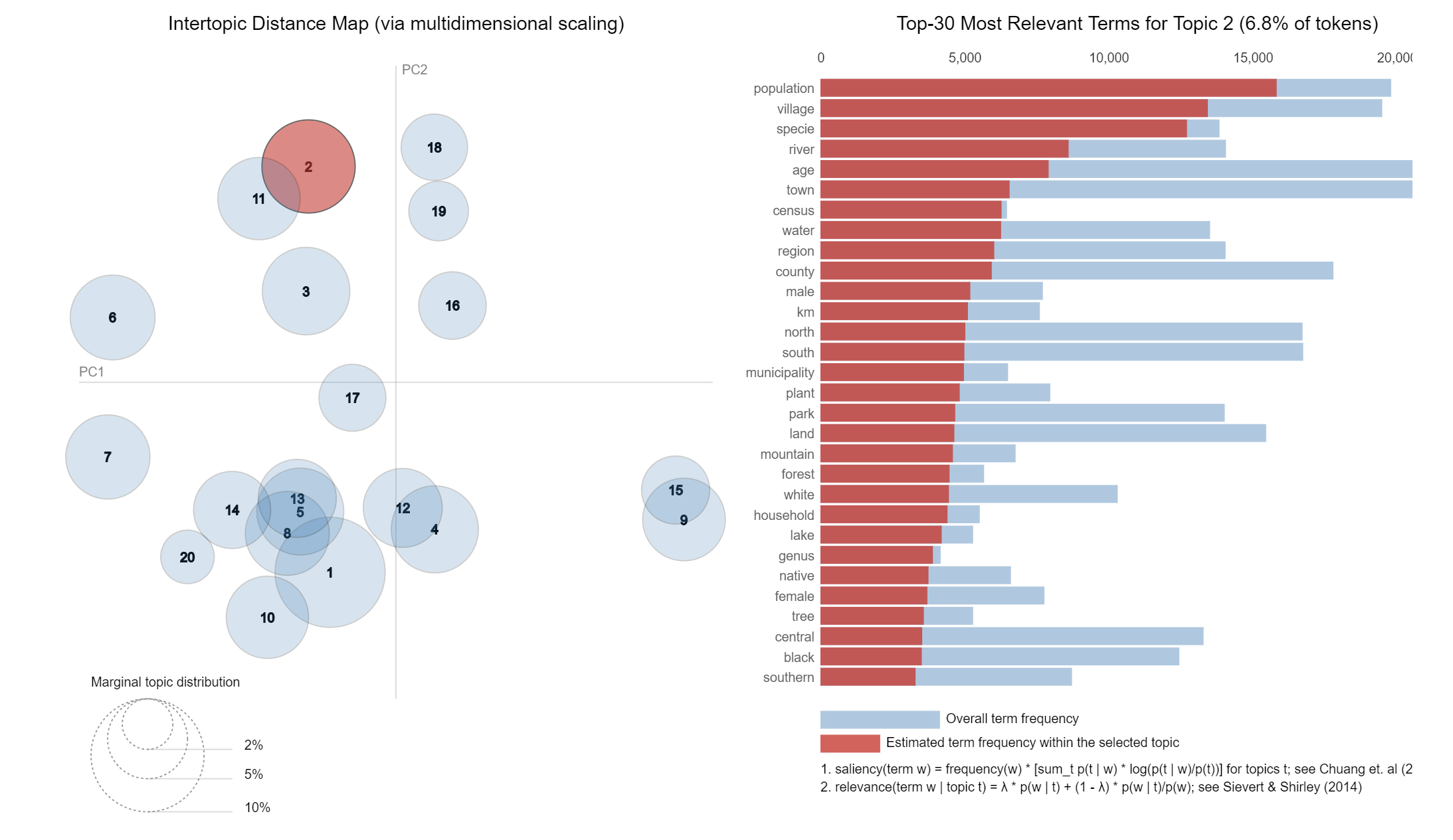
Findings
We spent a lot of time discussing how to infer the latent parameters of LDA. The final output that is actually of most interest is the topic vocab or beta. We ran our experiment on documents from Wikipedia and here are the vocabularies of the first two topics.